Vectorized Mandelbrot Rendering in MATLAB
Introduction
It is well known that describing calculations as linear algebra operations on vectors can result in much faster MATLAB code. Many times this is demonstrated on trivial examples that can be written as easily (or easier) in a vectorized form as they can be using loops. More complex cases often require more ingenuity and testing to make performant. Mandelbrot set rendering is a good example of an algorithm which is simple to specify as nested loops, but difficult to vectorize.
All profiling is done on an i9 12900KF processor, with 64GB DDR4 ram.
Mandelbrot Primer
The Mandelbrot set is the set of complex numbers $c$ for which the following iterative process does not diverge.
\[z_0 = 0\] \[z_{n+1} = z_n^2 + c\]Images of the set can be drawn by creating a grid of numbers spanning some region of the complex plain, and iterating using the above equation, testing if the magnitude $|z_n|$ exceeds some chosen “radius” in a given number of iterations. To draw more visually interesting pictures, often the points exterior to the set are colored according to the number of iterations before they escape this radius, or some other measure of the rate of divergence. For our purposes we will use this formula to color points outside the set.
\[\mu = n + 1 - \log(\log(|z_n|))/\log(2)\]See here for a derivation and further discussion of this formula. I make the following simplifications for ease of calculation. (avoiding extra division and taking a square root)
\[\mu = n + 1 - \log_2(\log(|z_n|^2)/2)\]This approach has 2 major benefits.
- The otherwise discrete integer iteration count is transformed into a continuous value, which results in nicely blended colors in the final image.
- The resulting coloring is independent of the chosen values for maximum iteration limit and escape radius. This allows certain optimizations we will discuss later.
Technically, the absolute largest the escape radius needs to be is 2, however the escape normalization is really an approximation that gets more accurate as the escape radius increases. For this testing I found that using an escape radius of 10 provided consistent enough results.
This is really all you need to know about Mandelbrot set rendering for making “shallow” images. There are many more computational details and algorithmic optimizations which become increasingly important for rendering small and detailed regions of the set, but these are beyond the scope of this article.
This algorithm is also inherently very parallelizable, since every point can be iterated completely independently. We are going to ignore that aspect for now and look at optimizing just a single thread of execution.
Setup
In order to draw the Mandelbrot set, we need some utility functions to create the complex grids that our rendering functions will take as input. For given real and imaginary bounds and desired resolutions, makeGrid returns the complex grid.
function [x, y, c] = makeGrid(x, y, xResolution, yResolution)
    x = linspace(x(1), x(2), xResolution);
    y = linspace(y(2), y(1), yResolution);
    c = flipud(x + 1i * y.');
end
The function squareZoom wraps the more general makeGrid and allows specifying a square region of the complex plain with only a complex center point and radius.
function [x, y, c] = squareZoom(center, radius, resolution)
    x = [real(center) - radius, real(center) + radius];
    y = [imag(center) - radius, imag(center) + radius];

    [x, y, c] = makeGrid(x, y, resolution, resolution);
end
We will start by rendering a zoomed out overview of the entire set, centered on the real axis. Each test image will have 1,000,000 pixels total (1000 by 1000).
[x, y, c] = squareZoom(-0.75, 1.25, 1000);
For Loop Baseline
Each rendering function will take an array of complex values, c, a maximum iteration limit, and an escape radius. They will return arrays containing the final iteration counts and magnitudes for each point in c. The simplest approach is to write a for loop over all of the points in c, inside of which is a while loop that exits when the magnitude of the point exceeds the escape radius of the iteration count exceeds the maximum limit, at which point we save the final iteration count and magnitude to the output arrays.
function [iterations, magnitudes] = loopMandel(c, maxIter, escape)

    iterations = zeros(size(c));
    magnitudes = zeros(size(c));

    for point = 1:numel(c)
        z = 0;
        z_magnitude = 0;
        iteration = 0;
        constant = c(point);
        while z_magnitude < escape && iteration < maxIter
            z = z*z + constant;
            z_magnitude = z*conj(z);
            iteration = iteration + 1;
        end
        iterations(point) = iteration;
        magnitudes(point) = z_magnitude;
    end
end
The colorization is handled by a function called normalizeEscape, which will be shared across all the rendering tests. Points that are in the Mandelbrot set will have squared magnitudes less than 4, and are assigned the darkest color in the colormap.
function mu = normalizeEscape(iterations, magnitudes)
    mu = zeros(size(iterations));
    escaped = magnitudes >= 4; % points that don't escape are left as 0
    mu(escaped) = ...
        iterations(escaped) + 1 - log2(log(magnitudes(escaped))/2);
end
Finally the mu array is scaled to the color map and saved to a png. I add an extra log transform to lighten the colors somewhat.
function saveRender(mu, filePath)
    % color scaling
    l = log10(mu);
    finite =~isinf(l);
    a = min(l(finite), [], 'all');
    b = max(l(finite), [], 'all');
    l = (l - a) ./ (b - a);
    l(~finite) = 0;
    l = l * size(jet, 1);
    % write to image, with jet colorscheme
    imwrite(l, jet, filePath);
end
Here are the function calls to create the image file. For this analysis, I am only going to profile the computational part of the process by timing the rendering function. We will use the same complex plain grid for testing all the versions of the rendering algorithm. An iteration limit of 1000 seems sufficient for this region.
tic();
[iterations_loop, magnitudes_loop] = loopMandel(c, 1000, 100);
toc()

mu_loop = normalizeEscape(iterations_loop, magnitudes_loop);
saveRender(mu_loop, 'loopMandelbrot.png');

Elapsed time is 2.774115 seconds.
The for loop approach is fairly concise, it is essentially just a one to one implementation of the mathematical description we started with, mapped over some collection of points. Unfortunately this clear code is much slower than it should be for the amount of work being done, clocking in at about 2.7 seconds. If we want better performance in MATLAB, we are going to have to vectorize.
Vectorization
Instead of expressing the computational work of our algorithm one scalar point at a time, we need to work with many points at once, allowing us to take advantage of builtin MATLAB functions to do the inner loop at a lower level than we have access to in our program. The difficulty here is that the amount of work that needs to be done per pixel is not the same, it depends on the pixels position relative to the set. We cannot simply specify the same operations on the entire array of complex points. Instead, we need a way to specify the group of points which have not yet escaped and must be iterated further.
Lets start with a rather naive attempt at vectorization, which directly translates all of the loop values into arrays, and works on the arrays using a list of indices which corresponds to the unescaped pixels. The array index will keep a list of unescaped points, and shrink as the render completes. When index is empty we are finished.
function [iterations, magnitudes] = naiveVecMandel(c, maxIter, escape)

    % allocate
    z = zeros(size(c));
    iterations = zeros(size(c));
    magnitudes = zeros(size(c));

    % indices of unifinished points
    index = 1:numel(c);

    % loop all the pixels at once
    while ~isempty(index)

        % iterate all unfinished points
        z(index) = z(index).*z(index) + c(index);

        % update iteration counts and magnitudes
        iterations(index) = iterations(index) + 1;
        magnitudes(index) = z(index).*conj(z(index));

        % keep only the unfinished indices in index
        index = index(...
            magnitudes(index) < escape & iterations(index) < maxIter);
    end
end
Elapsed time is 6.206970 seconds.
This version is much slower than the for loop implementation, even though its should be close to an exact vectorized translation of the same operations, plus some overhead for copying index every iteration. Unfortunately, MATLAB is closed source and most of the time detailed documentation on internal implementation is unavailable. Even after years of using it, its not exactly clear to me whether the interpreter/compiler can perform something like z(index) = z(index).*z(index) + c(index); as one loop without allocation or three with intermediate allocation. It is even less clear when it comes to multiple indexing operations across multiple lines. This situation may just be too complicated for MATLAB to refactor the code into something less redundant. As an experiment, lets explicitly copy from z into a new array and write back to it after each iteration.
function [iterations, magnitudes] = copyVecMandel(c, maxIter, escape)

    % allocate
    z = zeros(size(c));
    iterations = zeros(size(c));
    magnitudes = zeros(size(c));

    % indices of unifinished points
    index = 1:numel(c);

    % loop all the pixels at once
    while any(index, 'all')

        % copy values to avoid some redundant indexing
        z_tmp = z(index);

        % iterate all unfinished points
        z_tmp = z_tmp.*z_tmp + c(index);
        z_mag = z_tmp .* conj(z_tmp);

        % update iteration counts and magnitudes
        iterations(index) = iterations(index) + 1;
        magnitudes(index) = z_mag;

        z(index) = z_tmp;

        % keep only the unfinished indices in index
        index = index(...
            z_mag < escape & iterations(index) < maxIter);
    end
end
This is slightly faster!
Elapsed time is 4.703532 seconds.
It seems that copying memory to avoid redundantly indexing arrays is a good tradeoff here. We can use this idea to make a much more performant version of this algorithm. First, notice that we don’t really need the full z array, and we waste time indexing it twice every iteration. Instead, we can use the same pattern as we do for index, keeping a running list of points we are working on and discarding finished points as we go. We will still copy all the unfinished points every iteration, but we avoid indexing arrays. The same principle can be applied to the points in c. We are also redundantly updating the magnitudes and iterations arrays every iteration, since we only really need to store those values when the points are finished. In fact, we are doing a lot of redundant work to update iterations, when the values all change in sync. Combining all of these insights results in the following improved version.
function [iterations, magnitudes] = betterVecMandel(c, maxIter, escape)

    % allocate
    iterations = zeros(size(c));
    magnitudes = zeros(size(c));

    % indices of unfinished points
    index = 1:numel(c);

    % points that have yet to escape
    unfinished_z = zeros(numel(c), 1);
    unfinished_c = c(:);

    % loop all the pixels at once
    iteration = 0; % single iteration count
    while ~isempty(index)

        % perform one iteration
        unfinished_z = unfinished_z.*unfinished_z + unfinished_c;
        iteration = iteration + 1;

        % if we exceed the max iteration count, we are done
        if iteration >= maxIter
            iterations(index) = iteration;
            break;
        end

        % calculate magnitudes
        z_magnitude = unfinished_z.*conj(unfinished_z);

        % which of the current points have escaped?
        unfinished = z_magnitude < escape;
        finished = ~unfinished;
        finished_index = index(finished);

        % store the finished iterations and magnitudes
        iterations(finished_index) = iteration;
        magnitudes(finished_index) = z_magnitude(finished);

        % reduce the work load to the unfinished points
        index = index(unfinished);
        unfinished_z = unfinished_z(unfinished);
        unfinished_c = unfinished_c(unfinished);
    end
end
Elapsed time is 1.905352 seconds.
This version is much more verbose and includes a lot of extra logic, but runs faster than the simple loop implementation. It performs extra memory copies, but the amount of copying shrinks over time, and MATLAB seems to be able to do this kind of copying quickly. Lets use the matlab profiler to see how much time is spent in each part of the program.
profile on
[iterations_vec, magnitudes_vec] = betterVecMandel(c, maxIter, 100);
profile viewer
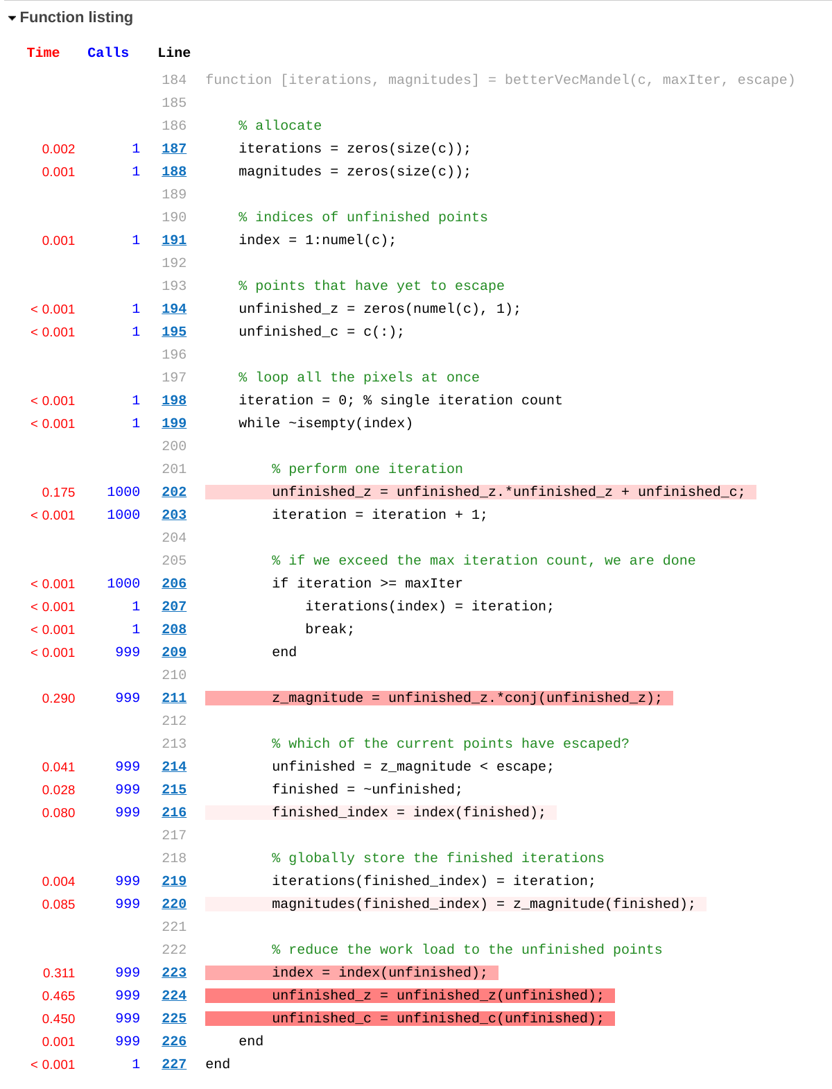
Here we can see how much time is spent on each line of the function. The actual calculation to iterate the points takes very little time compared to calculating the magnitudes of the points and performing the memory copies of the unfinished points. This is indicative of all the extra work needed to specify the computation in a way that MATLAB can execute efficiently.
Every programming language is a kind of virtual machine. The instructions provided by source code map to abstractions in the language, and the costs of the corresponding mechanisms in the runtime can be as important to performance as the physical hardware of the machine. The wrong system of abstractions at the language level can add to the complexity of writing code that performs well on the machine, and of course abstractions that conflict with optimal use of the underlying hardware will reduce the maximum achievable performance. In this case the memory copying is completely unnecessary at the hardware level, but is worth the cost there to be able to use the faster language level abstraction. For these reasons “higher level” languages often get a bad rap. Critics of abstraction argue that you should just use constructs that correspond more closely to the physical hardware if you care about performance. I think that improving performance of our languages without sacrificing ease of expression is a noble pursuit and should not be abandoned because of some less than perfect implementations so far. The association of expressive abstractions and slow, runtime interpreted languages is to some degree a quirk of historical circumstances rather than a fundamental limitation.
Further Improvement
There’s one more trick we can use to further improve the performance. Recall that the normalization formula we use allows the final result to be (approximately) independent of the escape radius and maximum iteration limit. This means that we can actually perform more iterations than strictly needed on each point without significantly effecting the final image. Since iterating the points is fast, but checking the escape conditions and removing finished points is slow, we can simply perform many iterations in a “batch” and only check for escaped points every so often. Here is the implementation.
function [iterations, magnitudes] = batchVecMandel(c, maxIter, escape, batchSize)

    % allocate
    iterations = zeros(size(c));
    magnitudes = zeros(size(c));

    % indices of unfinished points
    index = 1:numel(c);

    % points that have yet to escape
    unfinished_z = zeros(numel(c), 1);
    unfinished_c = c(:);

    % loop all the pixels at once
    iteration = 0; % single iteration count
    while ~isempty(index)

        % perform a batch of iterations on all unfinished points
        for batch = 1:batchSize
            unfinished_z = unfinished_z.*unfinished_z + unfinished_c;
        end
        iteration = iteration + batchSize;

        % if we exceed the max iteration count, we are done
        if iteration >= maxIter
            iterations(index) = iteration;
            break;
        end

        % calculate magnitudes after the batch is finished
        z_magnitude = unfinished_z.*conj(unfinished_z);

        % which of the current points have escaped?
        unfinished = z_magnitude < escape;
        finished = ~unfinished;
        finished_index = index(finished);

        % globally store the finished iterations
        iterations(finished_index) = iteration;
        magnitudes(finished_index) = z_magnitude(finished);

        % reduce the work load to the unfinished points
        index = index(unfinished);
        unfinished_z = unfinished_z(unfinished);
        unfinished_c = unfinished_c(unfinished);
    end
end
This simple change drastically improves performance.
Elapsed time is 0.402950 seconds.
Here I am using a batch size of 7, which appears to be the maximum for this region and level of zoom. Higher batch sizes can cause points which escape quickly to blow up and become infinite before they can be marked as finished. The upside is the more minimum iterations a region requires to render, the higher the maximum safe batch size should be.
The final result looks identical to before.

Here is the absolute magnitude difference between the batched and non batched outputs.
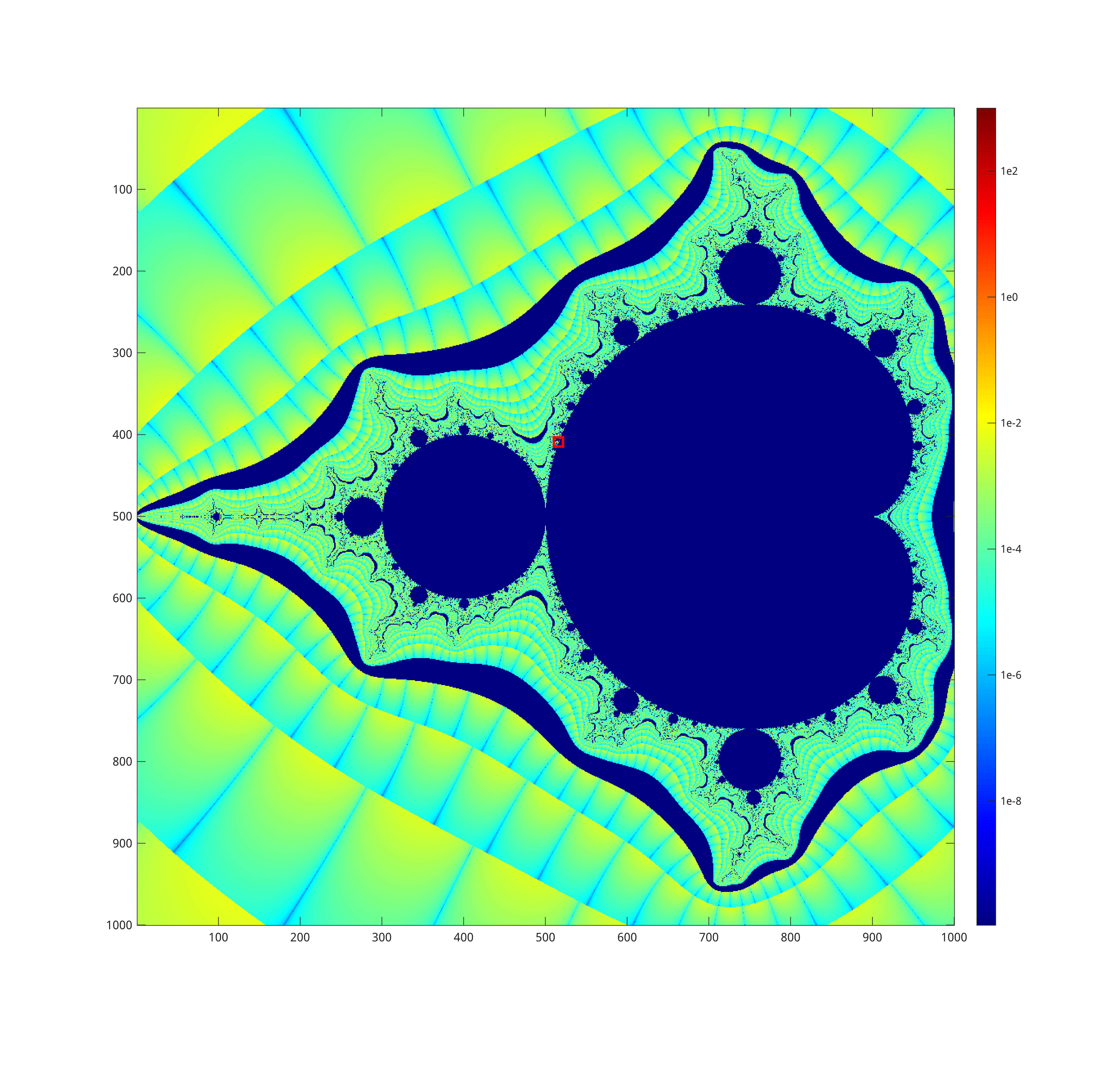
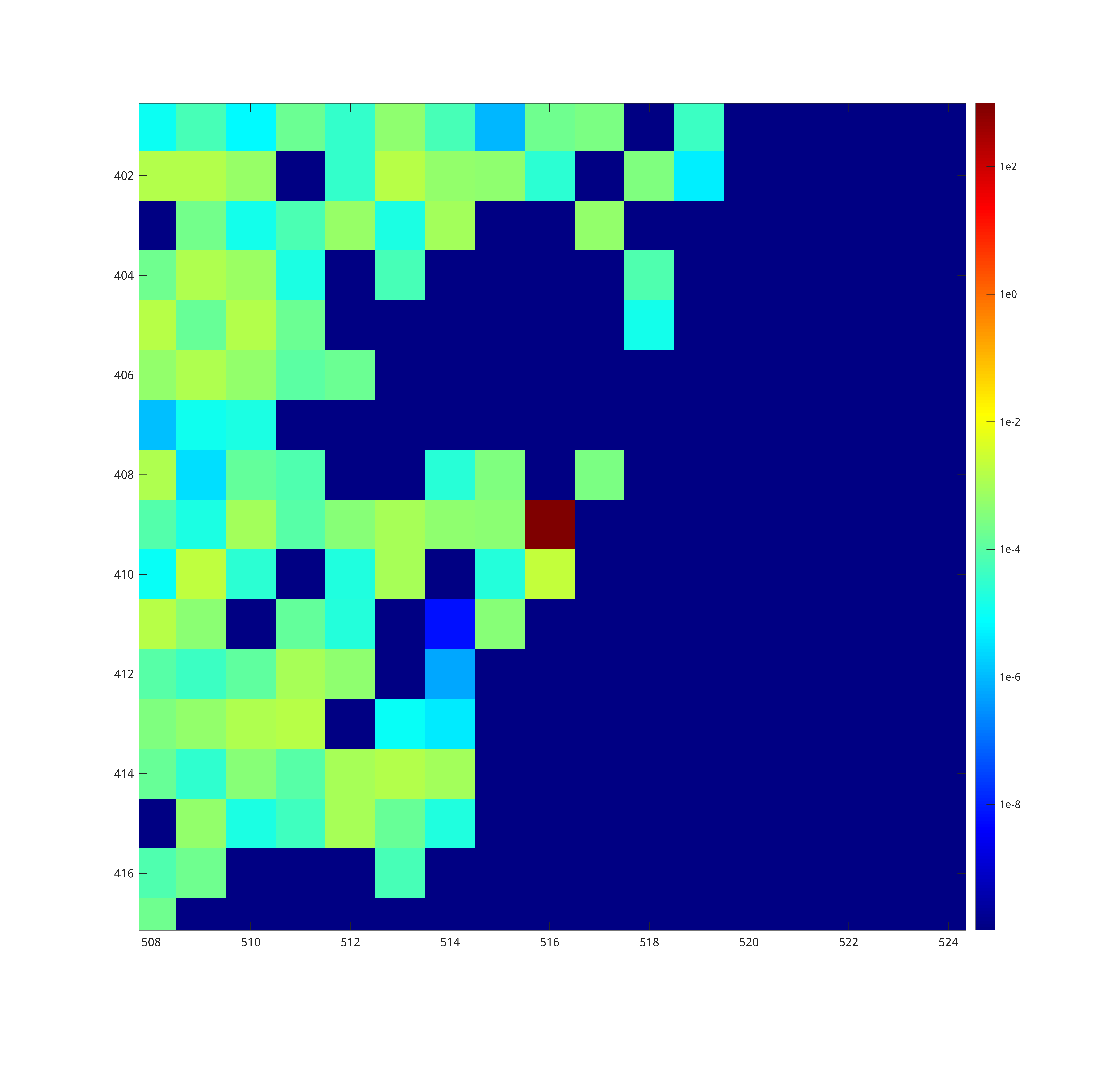
Most differences of this magnitude will be rounded to the same color in the 256 element colormap. The only major differences can occur at the border of the set, where a point can be erroneously classified as interior or exterior, since we are not checking for escape every iteration. I’ve highlighted the only pixel where this occurs in this image with a red box, and zoomed in to that area below.
It is important to keep in mind that all finite Mandelbrot renders are approximations of the true mathematical set. As long as there are not major distortions this level of inaccuracy is more than acceptable.
Conclusion
This new rendering code can be used to create images of more interesting regions of the mandelbrot set, such as this one that needs around 50,000 maximum iterations to draw the boundary of the set clearly.
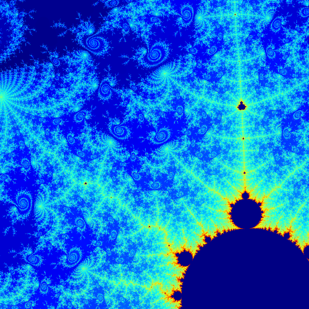
Elapsed time is 10.973643 seconds.
Unfortunately, this single threaded performance is still too slow to do serious deep zooms. Some of the necessary algorithm optimizations would be even more challenging to write in this vectorized way, as they require even more complicated logic per point. I hope to find time to write about some of those techniques in a future post.
I’ve written some very efficient parallel renders in Julia that can zoom in past double precision float limits and render 4k images of regions with maximum iterations limits in the tens of millions. Julia’s syntax and JIT compilation handles vectorization of functions automatically, enabling a lot of performance gains with minimal effort. This compilation stage also allows writing the same code to target both the cpu (parallel and single threaded) and gpu, while MATLAB requires using different constructs (and a paywalled library) for each. Ultimately I think Julia’s approach is the future of performant high level dynamic languages.
Creating a more efficient Mandelbrot renderer in MATLAB has been an interesting exercise. Some of these optimizations only really make sense in this specific language, but the idea of batching iterations and limiting magnitude calculations might be more widely applicable. Applying this for each parallel execution thread could result in significant speed ups. In the future I may try to adapt this technique to my deep rendering suite in Julia.